使用CIRCLIZE对VCF文件作图

R package circlize:可惜这个文档写得太枯燥。下面作图主要参考这个教程Variant Visualisation

我们的目的是使用CIRCLIZE这个程序来对VCF文件作图，即对VCF进行简单的可视化，显示SNP或INDEL在染色体上的位置。

> library(circlize)

# SNV
> snp=read.table("./snp.vcf")
> snv=cbind(snp[,1],snp[2],snp[,2]+1)
# INDEL
> indel=read.table("./indel.vcf")
> indels=cbind(indel[,1],indel[2],indel[,2]+1)
# PLOT
> circos.clear() # 确保在作图之前circos是关闭状态，若首次作图，不必运行
> x11() # 加载x11() DEVICE，对比发现，作图速度会快很多
> par(mar = c(1, 1, 1, 1))
> circos.par("start.degree" = 90)
> circos.par("track.height" = 0.1)
> circos.par("canvas.xlim" = c(-1.3, 1.3), "canvas.ylim" = c(-1.3, 1.3))
#circos.initializeWithIdeogram(species = "hg19")
> circos.initializeWithIdeogram(species = "hg38") # 确保参考基因组版本正确
#------------------------------------------
# 1st Layer
> circos.genomicTrackPlotRegion(snv,stack=TRUE, panel.fun = function(region, value, ...) {
  circos.genomicPoints(region, value, cex = 0.05, pch = 9,col='orange' , ...)
})
# 2nd Layer
> circos.genomicTrackPlotRegion(indels,stack=TRUE, panel.fun = function(region, value, ...) {
  circos.genomicPoints(region, value, cex = 0.05, pch = 9,col='blue' , ...)
})
# TITLE & LEGEND
> title("Somatic calls (SNV-INDEL)") # 添加标题
> legend(0.7,1.4,legend=c("SNV", "INDEL"),col=c("orange","blue"),pch=c(16,15),cex=0.75,title="Tracks:",bty='n') # 添加图例
> circos.clear() # 关闭设备

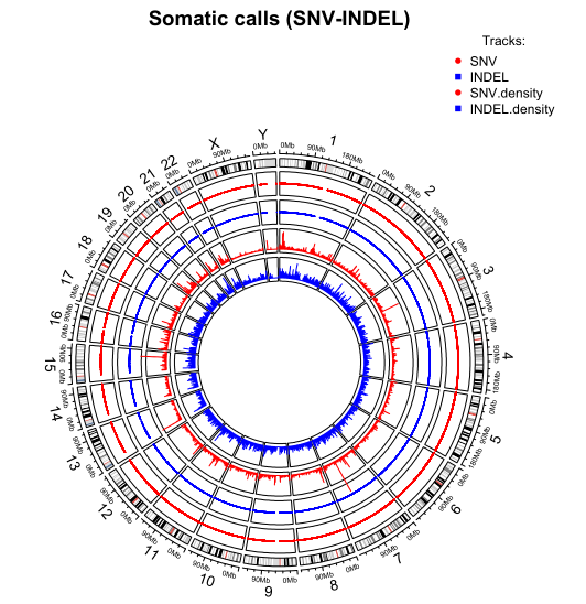
上面在作图时，实际上我们只标示了在染色体何位置上有SNP或INDEL，但不能显示差异，我们还可以对SNP或INDEL的密度作图，计算密度可以使用VCFTOOLS，

> vcftools --vcf snp.vcf --SNPdensity 100000 --out snp
# 生成两个文件：snp.snpden & snp.log
> vcftools --vcf indel.vcf --SNPdensity 100000 --out indel
# 生成两个文件：indel.snpden & indel.log

回到R中，

> snpden <- read.table("./snp.snpden",sep="\t",header=T)
> head(snpden)
  CHROM BIN_START SNP_COUNT VARIANTS.KB
1  chr1         0         8        0.08
2  chr1    100000        16        0.16
3  chr1    200000         2        0.02
4  chr1    300000         0        0.00
5  chr1    400000         0        0.00
6  chr1    500000         0        0.00

# 需要注意一下，如果CHROM中包含chr1:chr22,chrX,chrY以外的染色体，需要将其去掉，否则会报错
> head(table(snpden$CHROM))

                  chr1 chr1_KI270706v1_random chr1_KI270709v1_random 
                  2490                      2                      1 
chr1_KI270710v1_random chr1_KI270711v1_random chr1_KI270712v1_random 
                     1                      1                      1 

chr <- paste("chr",c(1:22,"X","Y"),sep="")
snpden2 <- snpden[snpden$CHROM %in% chr,]
snpden2 <- droplevels(snpden2)

# 3列与4列传递的信息是一致的，只保留1，2，4列即可
> snpden2 <- snpden2[,c(1,2,4)]
> head(snpden2)
  CHROM BIN_START VARIANTS.KB
1  chr1         0        0.08
2  chr1    100000        0.16
3  chr1    200000        0.02
4  chr1    300000        0.00
5  chr1    400000        0.00
6  chr1    500000        0.00

# 修改列名
> colnames(snpden2)<-c("Chr","X","Y")
> head(snpden2)
   Chr      X    Y
1 chr1      0 0.08
2 chr1 100000 0.16
3 chr1 200000 0.02
4 chr1 300000 0.00
5 chr1 400000 0.00
6 chr1 500000 0.00
# 现在，作图数据准备完成
> circos.trackPlotRegion(factors=snpden2$Chr,y=snpden2$Y)
> circos.trackLines(snpden2$Chr,snpden2$X,snpden2$Y*2,col="red",lwd=0.2) # 此处，对snpden2$Y整体乘2，是为了突出显示，根据需要决定是否保留

对于INDEL，也是如此，

> indelden <- read.table("./indel.snpden",sep="\t",header=T)
> head(indelden)

# chr <- paste("chr",c(1:22,"X","Y"),sep="")
> indelden2 <- indelden[indelden$CHROM %in% chr,]
> indelden2 <- droplevels(indelden2)

> indelden2 <- indelden2[,c(1,2,4)]
> head(indelden2)
> colnames(indelden2)<-c("Chr","X","Y")
> head(indelden2)

> circos.trackPlotRegion(factors=indelden2$Chr,y=indelden2$Y)
> circos.trackLines(indelden2$Chr,indelden2$X,indelden2$Y,col="blue",lwd=0.2)

# 最后，加上标题与图例
title("Somatic calls (SNV-INDEL)")
legend(0.7,1.4,legend=c("SNV", "INDEL","SNV.density", "INDEL.density"),col=c("red","blue","red","blue"),pch=c(16,15,16,15),cex=0.75,title="Tracks:",bty='n')
circos.clear() # 退出DEVICE