分析GSE100666,6个配对样本,平台是GPL16951,分析过程如下:
1 | setwd("D:/GEO") |
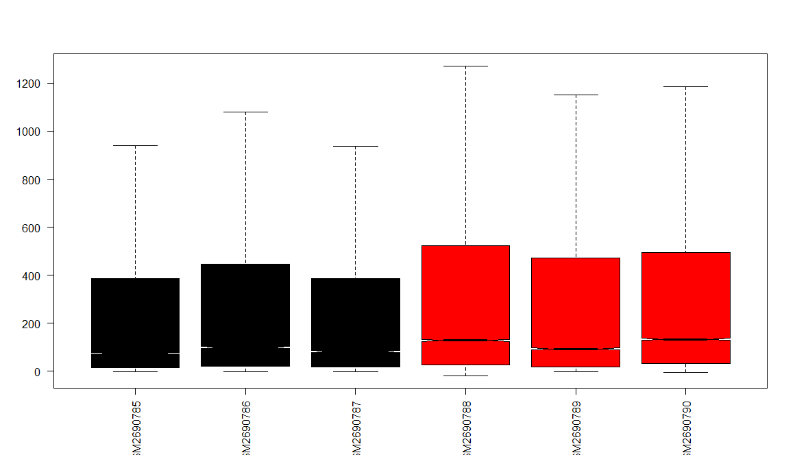
1 | # NORMALIZATION ---- |
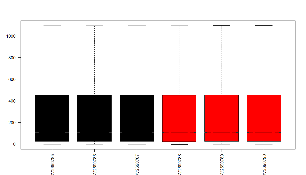
1 | # LOG2 TRANSFORM ---- |
1 | # COMBINE PLOT ---- |
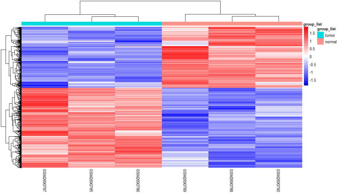
1 | # HEATMAP ---- |
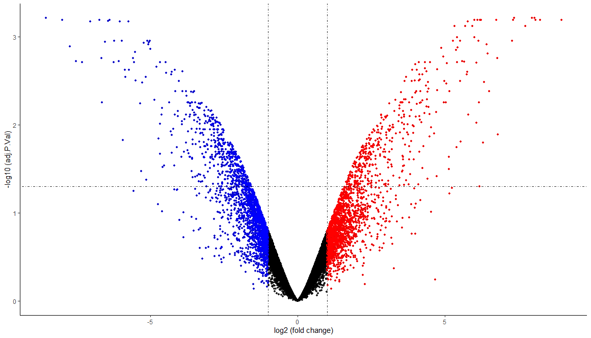
1 | # VOLCANO PLOT ---- |
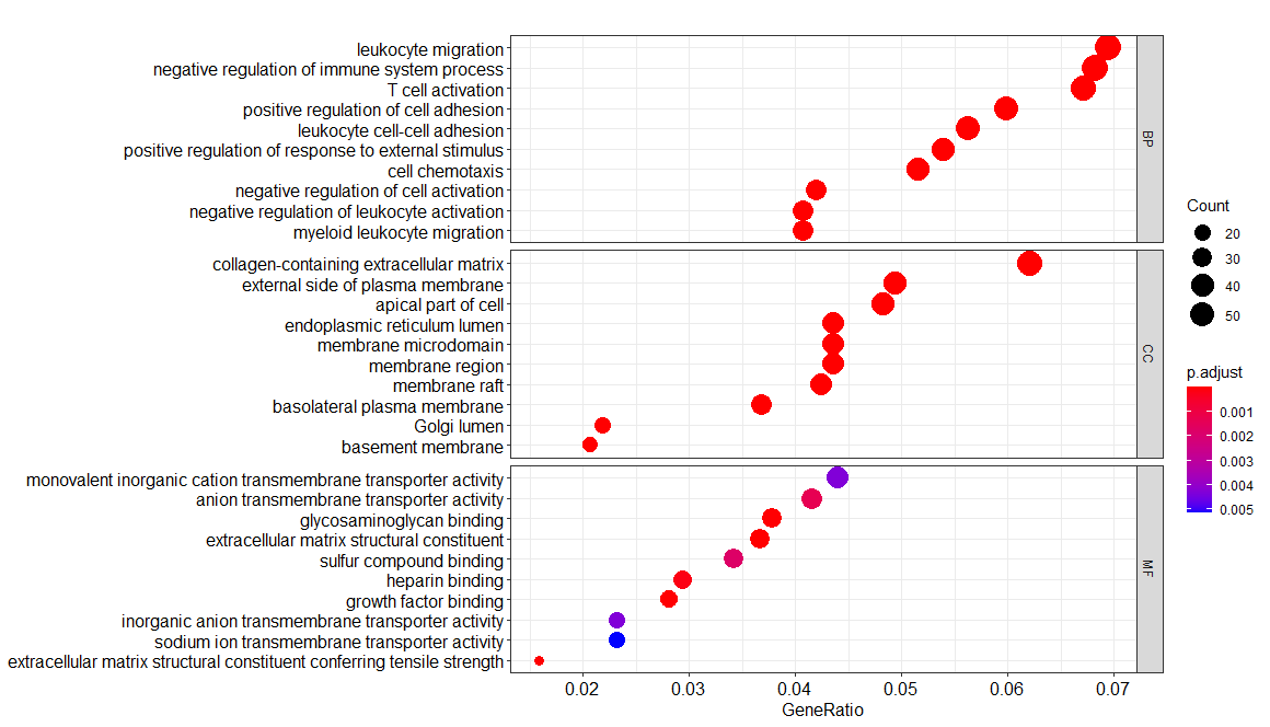
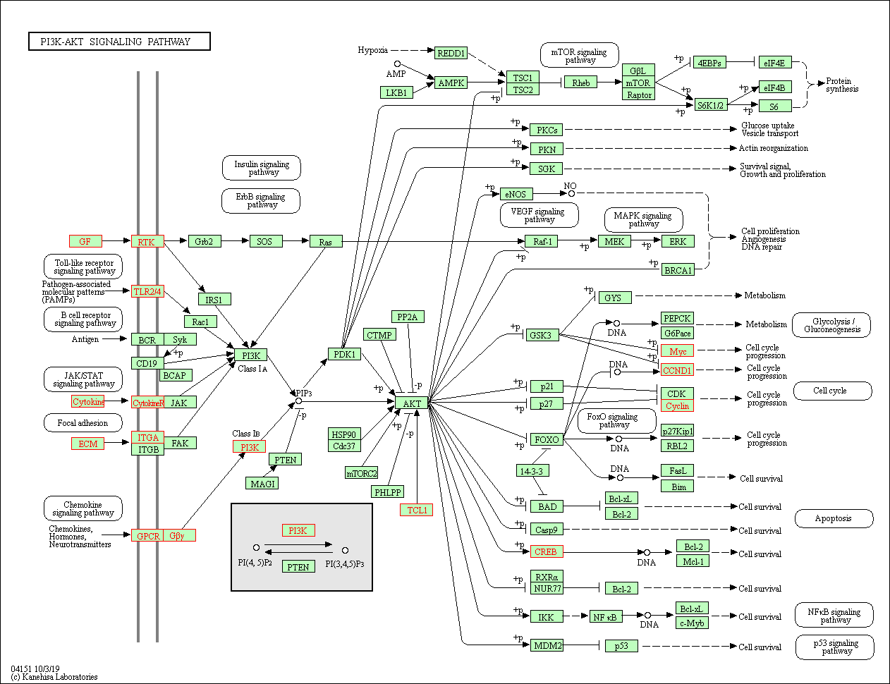
1 | # ENRICH |
1 | EGG <- enrichKEGG(gene= gene$ENTREZID, |
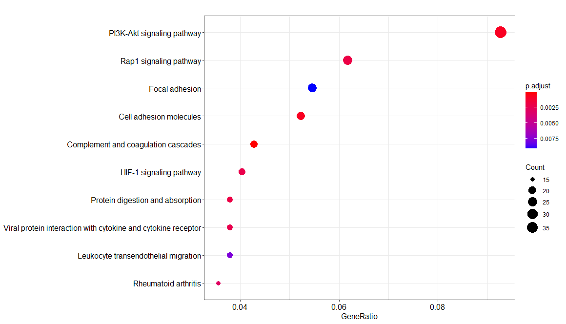
1 | test <- data.frame(EGG) |
分析GSE100666,6个配对样本,平台是GPL16951,分析过程如下:
1 | setwd("D:/GEO") |
1 | # NORMALIZATION ---- |
1 | # LOG2 TRANSFORM ---- |
1 | # COMBINE PLOT ---- |
1 | # HEATMAP ---- |
1 | # VOLCANO PLOT ---- |
1 | # ENRICH |
1 | EGG <- enrichKEGG(gene= gene$ENTREZID, |
1 | test <- data.frame(EGG) |